None .. An html document created by ipypublish

outline: ipypublish.templates.outline_schemas/rst_outline.rst.j2 with segments: - nbsphinx-ipypublish-content: ipypublish sphinx content

10. Course exercises

Basile Marchand (Materials Center - Mines ParisTech / CNRS / PSL University)

10.1. Slicing exercise

1. create the string: I love python and numpy! 1.access the first and last character of the string ‘I’ and ‘!’

2. cut the chain to keep only “love”

3. reverse the chain:! ypmun dna nohtyp evol I

4. cut the chain to keep only “Ilv pto ad nmy”

10.2. Exercises on strings

10.2.1. Exercise 1

1. create a string in python

2. print the string and its length using an f-string

3. create another character string

4. concatenate the two strings

5. put the result in uppercase

10.2.2. Exercises 2

1. create a multi-line string and display it

2. split the string to obtain a list of lines (split method)

3. display each line using a for loop by prefixing it with its number

10.3. Exercise on the lists

1. build a list containing an integer, a character string, a float, a boolean

2. modify the first element of the list

3. slice the list so as to keep only one element out of 2 from the beginning

4. test if an element is in the list

5. create a new list containing a list itself

6. concatenate the two lists

7. print with a for the elements of the list

10.4. Exercise on dictionaries

1. create a dictionary with pairs of people described by name and age

2. display the type of a dictionary

3. test if a person is in the dictionary and if so modify his age

4. Apply the items function to the dictionary, what does it return?

5. print with a for the names and ages of all the people in the dictionary

10.5. Exercises on functions

10.5.1. Exercise 1

The objective of this first exercise is to carry out a Python program allowing an elementary examination of a large number of experimental results. The experimental tests in question are tensile tests on test specimens.

The points of interest that are discussed in this exercise are as follows:

1. Modularity of the code.

2. Processing of text files

3. Simple math function

The expected operation for the program is as follows:

1. The user provides as input the path to the folder containing all the experimental files

2. The program lists all the files contained in this folder

3. For each file: Reading data from file Identification of maximum stress and strain at break

   • Storage of these quantities in a container

4. Calculation of the means of the maximum stress and the breaking stress

5. Calculation of the variances of the maximum stress and the breaking stress

6. Display of results in the console (with its own formatting)

7. Write the results in a text file.

The files containing the experimental data can be downloaded at the following address http://bmarchand.fr/download/data/tp1.tar.gz

10.5.2. Exercise 2

In this second exercise the objective is to define an evalPolynom function which must allow:

1. Evaluate an arbitrary order polynomial, defined by its coefficients, into a given x value.

2. Return, if the user requests it, the values ​​of M successively derived from this polynomial evaluated atx as well.

3. Display a clear help message via the help function

10.6. Exercises on the classes

10.6.1. Exercise 1

In this first exercise you will define a class Vector2D andVector3D having:

• for private attributes:

  • values a list of doubles (2 values ​​forVector2D and 3 values ​​for ̀Vector3D

  • size an integer specifying the size of the vector

The desired behavior for these two objects is as follows:

1. Be able to display the vector properly using print

2. Return the size using the len function

3. Access the values ​​contained in the values attribute

4. Have all the usual operations* Sum of two ̀Vector Difference of two ̀``Vector`` Term-to-term multiplication of two ̀Vector

5. Make broadcasting, i.e. the sum of a Vector2 and aVector3 must return a Vector3 for which the last component is unchanged.

10.6.2. Exercise 2

Note:

Don’t you find that the previous exercise still involves a lot of copy and paste? You should in any case !!!

The objective of this exercise is therefore to redo exercise 1 by using the concept of inheritance in order to minimize copy and paste.

10.7. Numpy exercise

10.7.1. Data manipulation

The objective here is to redo exercise 1 on functions by now using numpy as much as possible

10.7.2. Image manipulation (thanks V. Roy for the subject)

import numpy as np
from matplotlib import pyplot as plt

concepts involved in this lab

on numpy.ndarray arrays * reshape (), tests, boolean masks, ufunc, aggregation, linear operations on numpy.ndarray * the other concepts used are recalled (very briefly)

for reading, writing and viewing images * use plt.imread,plt.imshow * use plt.show() between two plt.imshow () in the same cell

note

• we use the basic functions on the pyplot images for simplicity

• we do not mean here at all that they are the best for example matplotlib.pyplot.imsave does not allow you to give the compression quality while the save function ofPIL allows it

• you are free to use another library like opencv if you know it well enough to get by (and install it), the pictures are just a pretext don’t forget to use the help in case of problem.

10.7.2.1. Sum of RGB values ​​of an image

0. Read the image media/les-mines.jpg

1. Create a new array numpy.ndarray by adding with the operator``+`` the RGB values ​​of the pixels of your image

2. Display the image (not terrible), its maximum and its type

3. Create a new array numpy.ndarray by adding with the aggregation function``np.sum`` the RGB values ​​of the pixels of your image

4. Display the image, its maximum and its type

5. Why this difference? Use the help np.sum?

6. Make the image grayscale of type 8-bit unsigned integer (whichever way you prefer)

7. Replace in the grayscale image, values> = to 127 by 255 and those lower by 0 Display the image with a grayscale color map you can use the numpy.where function

8. with the function numpy.unique look at the different values ​​you have in your black and white image

10.7.2.2. Sepia image

To change the R, G and B values ​​of a pixel to sepia (encoded here on an 8-bit unsigned integer)

1. we transform the values \(R\), \(G\) and \(B\) by the transformation \(0.393\, R + 0.769\, G + 0.189\, B\) \(0.349\, R + 0.686\, G + 0.168\, B\) \(0.272\, R + 0.534\, G + 0.131\, B\) (attention the calculations must be done in floats not in uint8 so as not to have, for example, 256 becoming 0)

2. then we threshold the values ​​which are greater than 255 to255

3. of course the image must then be submitted in the correct format (uint8 or float between 0 and 1)

Exercise

1. Make a function which takes an RGB image as argument and renders a sepia RGB image.

2. Spend your patchwork of colors in sepia Read the media/patchwork-all.jpg file if you don’t have a custom file

3. Pass the image media/les-mines.jpg in sepia

10.7.2.3. Image compression by SVD

In this exercise the objective is to compress a grayscale image using an SVD (Singular Value Decomposition). The image to compress is as follows:

Fig. 10.7.1 data/carrie_fisher.png

As a reminder, the SVD decomposition of a \(\mathbf{A} \in \mathbb{R}^{m\times n}\) matrix is ​​written as follows:

\[\mathbf{A} = \mathbf{U}\cdot\mathbf{\Sigma}\cdot\mathbf{V}\]

With \(\mathbf{U}\in \mathbb{R}^{m\times m}\), \(\mathbf{\Sigma}\in\mathbb{R}^{m\times n}\) is a diagonal matrix of singular values ​​and \(\mathbf{V} \in \mathbb{R}^{n\times n}\).

Question 1:

Load the image of Carrie Fisher (you will find in the data folder a file carrie_fisher.npy containing the image or in the form of an np.ndarray) and calculate its decomposition into singular values.

Question 2:

Trace the evolution of the singular values ​​of the image.

Question 3:

For different truncations (\(k=\lbrace 1,5,10,15,20,30,50,100 \rbrace\)) reconstruct the image, display it and calculate the compression rate obtained.

10.7.2.4. Solving a system of N springs

from IPython.display import IFrame

IFrame("./media/spring.pdf", width=600, height=300)

<IPython.lib.display.IFrame at 0x7ff0de5ec390>

The objective is to determine by a matrix approach the response of the system to a \(F\) effort.

The formulation of the problem must therefore be reduced to the resolution of a problem of the form

\[\mathbf{K} \cdot \mathbf{u} = \mathbf{F}\]

With \(\mathbf{K} \in \mathbb{R}^{M\times M}\), \(\mathbf{u} \in \mathbb{R}^{M}\), \(\mathbf{F} \in \mathbb{R}^{M}\) and \(M\) the number of points in the system.

For that it is recalled that the potential energy of the system can be expressed in the following form:

\[E_p = \frac{1}{2} \sum_{i=1}^{N} \left( u_{i,1} - u_{i,0} \right)\cdot k_{i} \cdot \left( u_{i,1} - u_{i,0} \right)\]

With \(u_{i,0}\) the displacement of the first attachment node of the \(i\)-th spring and \(u_{i,1}\) the displacement of the second attachment node of the \(i\)-th spring.

This potential energy can be written in the following matrix form:

\[E_p = \frac{1}{2} \mathbf{U}^T \cdot \mathbf{K} \cdot \mathbf{U}\]

Then using the potential energy theorem we can write that

\[\mathbf{K}\cdot \mathbf{U} = \mathbf{F}\]

Question 1:

From the expression of the potential energy of a spring define the elementary stiffness matrix.

Question 2:

Use the stiffness matrix of a spring to build the global \(\mathbf{K}\) matrix. To do this, use the notion of connectivity table. As a reminder, the connectivity table is a \(L\) list such that the \(i\)-th element of \(L\) is the doublet of the indices of the spring attachment points.

Question 3:

Build the right hand side \(F\).

Question 4:

Solve the linear system

Bonus:

Using matplotlib, visualize the profile of the matrix \(\mathbf{K}\):

import matplotlib.pyplot as plt
plt.imshow (K)
plt.colorbar ()
plt.show ()

What can we conclude from this? What avenue of improvement is possible to accelerate the resolution of the problem?

10.8. Scipy exercises

10.8.1. EDO resolution

Consider a classical RC circuit defined by the following differential equation:

\[RC \frac{du}{dt} + u = u_e\]

\[\frac{du}{dt} = \frac{u_e - u }{RC}\]

With \(R=1000\Omega\), \(C=10^{-6}F\) and \(u(t=0) = 0\).

Question 1:

In the case where \(u_e(t) = U_0\) with \(U_0=10\,V\) calculate the solution of the differential equation over the interval \([0, 0.005]\).

Question 2:

In the case where \(u_e(t) = U_0 \sin \left( 2\pi f t \right)\) with \(U_0=10\,V\) and \(f=100\,Hz\) calculate the solution of the differential equation over the interval \([0, 5/f]\).

10.8.2. Solving a system of differential equation

Consider a classical RLC circuit defined by the following differential equation:

\[LC\frac{d^2u}{dt^2} + RC \frac{du}{dt} + u = u_e\]

Question 1:

Transform this second-order equation into a system of two first-order equations.

Question 2:

Determine the evolution of \(u(t)\) over the interval \(t \in [0, 0.02]\) for \(R=1000\,\Omega\), \(F=10^{-6}\,F\). It is up to you to choose the value of \(L\) to solve: (i) in pseudo-periodic regime; (ii) aperiodic; (iii) critical.

As a reminder :

\[\begin{split}q = \frac{1}{R} \sqrt{ \frac{L}{C} } \; ; \; \begin{cases} q = \dfrac{1}{2} & critical \\ q < \dfrac{1}{2} & aperiodic \\ q > \dfrac{1}{2} & pseudo-periodic \end{cases}\end{split}\]

If we want by using ipywidgets (we have to install it via conda) we can make an interactive graph with the value of \(L\).

10.8.3. Find the zero of a scalar function

Consider Kepler’s equation:

\[x - e\cdot \sin x = m\]

Question 1:

Using scipy find the solution of Kepler’s equation in the case where \(e=\frac{1}{2}\) and \(m=1\). Check that the solution found by scipy is correct.

10.8.4. Parameter identification — RC circuit

Consider the RC circuit previously studied.

We will try to identify the parameter R of the system from “experimental” data. The experimental data in question are given in the file notebook / data / exp _data_ rc.dat. If we represent these data we obtain the following curve:

import matplotlib.pyplot as plt
import numpy as np
import pathlib as pl

data = np.loadtxt(str(pl.Path(".") / "data" / "exp_data_rc.dat"))

plt.plot( data[:,0], data[:,1])
plt.xlabel("Time (s)")
plt.ylabel("U (V)")
plt.show()

Fig. 10.8.1 Code Cell Output

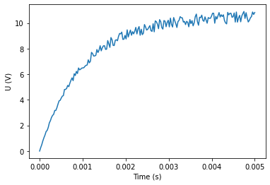
These data are obtained with the following configuration:

\[u_e = 10\,V\, ; \, C=10^{-6}\,F\, ; \, R=??\]

Question 1: Formulate the optimization problem to be solved to identify the parameter R?

Question 2: Using scipy.optimize identify the value of the R parameter.

Question 3: Represent on the same graph the experimental data and the result of the model for the identified value of \(R\).